Note
The following is a description of how to illustrate the branching geometry of algebraic functions using differential equation. Another more simple method is to compute and plot the associated Puiseux expansion of the branch. This is described in Section $6$ and $7$.Although algebraic functions are usually studied in the context of their normal Riemann surfaces, this discussion focuses on their real and imaginary plots over the complex plane.
A complex-valued function $f(z)=w$ of a complex variable $z=x+iy$ has a real part and imaginary part. We usually write this as $f(z)=u(x,y)+i v(x,y)$ with $u$ and $v$ real-valued functions of the real variables $x$ and $y$. The plots below illustrate portions of the real and imaginary components of the function studied in this exercise and one reason for separating out the real and imaginary components is that it is sometimes easier to study properties of a complex-valued function by restricting attention to either it's real or imaginary part. For example, it is easier to visualize contour integration over an algebraic function by studying the contour over the real part of the function.
Figure 1 is a function of degree 12 and although one customarily begins with a simple example when explaining a subject, this function was selected as a particularly beautiful example of an algebraic function with the hope that it's elegance will capture the interest of the reader so that they may wish to explore this subject further.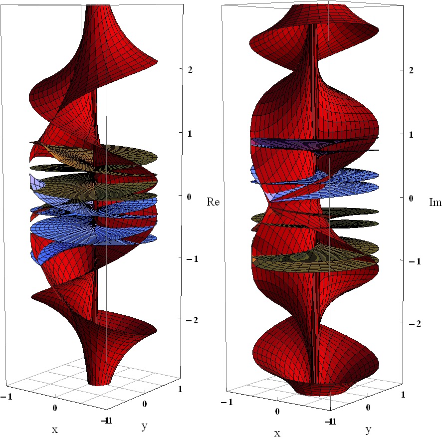
Although this discussion is written for the general reader having an introductory understanding of Calculus, a more thorough understanding of Calculus and Differential Equations would allow the reader greater comprehension of the subject.
The general form of an algebraic function $w(z)$ is given implicitly by $$ \begin{equation} f(z,w)=a_0(z)+a_1(z)w+a_2(z) w^2+\cdots+a_n(z)w^n=0 \end{equation} $$ where $a_i(z)$ is a polynomial function in $z$. For example, the square root function $w(z)=\sqrt{z}$ is given by the expression $f(z,w)=z-w^2$.We wish to consider the expression $$\frac{1}{w^4}\left(\frac{\overline{a}}{a} \frac{\left(a^2-w^2\right)}{\left(1-(\overline{a})^2w^2\right)}\right)^4=z,\quad a=2/3 e^{\pi i/3}$$ which can be written as $$ f(z,w)=a_1+a_2 w^2+(a_3+b_3z) w^4+(a_4+b_4 z) w^6+(a_5+b_5 z) w^8+a_6 z w^{10}+a_7 z w^{12}=0. $$ And our objective is to find $w(z)$. We will now focus on the real component of the function for the remainder of this discussion and display it separately in Figure 2 and now explain how to generate this plot. Remember the plot in Figure 2 is only a portion of the function chosen to nicely fit in the boundaries of the plot. The imaginary component is generated in an identical fashion. The method used is numerical integration around annular regions separated by singular points of the function. At the singular points, the function is not analytic so we must avoid those points. The function is singular when $f(z,w)=0$ and $\displaystyle \frac{df}{dw}(z,w)=0$. We can determine these points by the following Mathematica code:

A plot of the singular points in the $z$-plane is shown in Figure 4. Since there is a singular point at the origin and two on the unit disc, for this particular exercise, we will plot the function in a disc centered at the origin with radius $0\lt r \lt 1$.
Recall if we are given an implicit function $f(z,w)=0$ and wish to compute $\frac{dw}{dz}$, we have $$\frac{dw}{dz}=-\frac{\frac{df}{dz}}{\frac{df}{dw}}.$$ And if $z=g(r,t)$ as in the case over the complex plane where $z=re^{it}$, we have: $$ \begin{array}{cccc} \underline{\text{Azimuthal Equation}} & & & \underline{\text{Radial Equation}} \\ \displaystyle\frac{dw}{dt}=-\frac{\frac{df}{dz}}{\frac{df}{dw}}\frac{dz}{dt} & & & \displaystyle\frac{dw}{dr}=-\frac{\frac{df}{dz}}{\frac{df}{dw}} \frac{dz}{dr} \end{array} $$ Numerically integrating these two differential equations is the primary means of generating Figure 1 and this integration is easily accomplished in Mathematica. But in order to numerically integrate, we must first choose an initial value for the integration. We can pick the initial value by simply computing the twelve roots to $f(z,w)$ for some initial value $z_0$. Let's choose $z_0=1/2-1/2i$ since this point on the complex $z$-plane is easily identified in the figures (Black point in mesh lines of Figure 3). Using NSolve in Mathematica:
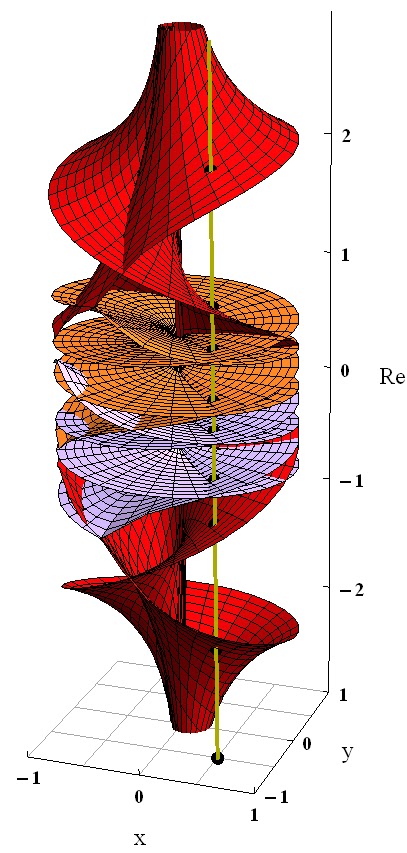
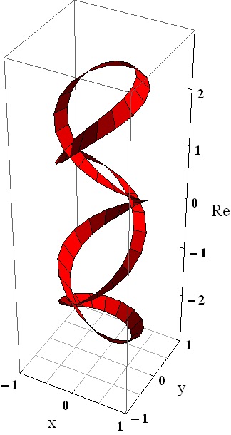
Illustrating algebraic functions in discs surrounding a singular point will produce surfaces which either fully wrap around themselves or "ramify" into distinct branches which wrap around themselves. In this example, the function ramifies into three such branches, color-coded red, purple, and gold in the figures, each wrapping around itself four times and even though the three branches in the figures seem to intertwine around each other, in the 4D-complex space they do not intersect. Figure 5 shows the three branches separated. We identify branches like these as "4-cycle" branches and in general, designate an algebraic branch of $w(z)$ wrapping around itself $n$ times as an $n$-cycle branch given by the expression $w_n(z)$. In this example, we have three $4$-cycle branches at the origin and can designate them as $w_{(4,1)},w_{(4,2)},w_{(4,3)}$.
| 2.0043-0.2869 i |
| 0.9121-2.8634i |
| 0.5545-0.8064i |
| 0.5347-0.1797i |
| 0.1325-09454i |
| 0.1211-0.3506i |
| -0.1211+0.3506i |
| -0.1325+0.9454i |
| -0.5347+0.1797i |
| -0.5545+0.8064i |
| -0.9121+2.8623i |
| -2.0043+0.2869i |

For example, let's focus on the red branch and the root on this branch identified in the first plot in Figure 5 at the yellow dot on the red surface. Recall $z_0=1/2-1/2i$ and the yellow dot on Figure 5 represents the location on the surface of this branch of the function, the real component of the root $w=2.0043-0.2869 i$. Now, in general we will not know which root corresponds to which branch until we have completed the integration but for this exercise, it if helpful to know beforehand in order to better understand the process.
We are now ready to integrate the function and thereby "traverse" the red branch. We will do this by numerically integrating the azimuthal equation over the function in a circular path by letting $z_0=1/2-1/2i$, $w_0=2.0043-0.2869 i$. and $z=\frac{1}{\sqrt{2}}e^{it}$ using the expression: $$\frac{dw}{dt}=-\frac{\frac{df}{dz}}{\frac{df}{dw}}\frac{dz}{dt}.$$
And after each $2\pi$ loop, we check if we have returned to $w_0$. If not, we integrate another $2\pi$ and continue this way until we have gone around $n$ times or reached $w_0$ whichever comes first. Using Mathematica, we write

The value of mysol will then be a numerical approximation to $w(z)$ for this particular branch of the function, in our case, over the red surface along a path with $z=\frac{1}{\sqrt{2}} e^{it}$. For example, suppose we wanted to know what the value of the function over the yellow path is when $t=\frac{\pi}{4}$? In Mathematica, we would use the command (w[t]/.mysol)/.t->PI/4. This would return $2.32574-1.18347i$. And if we likewise computed the 12 roots to the function for $z=\frac{1}{\sqrt{2}} e^{\pi i/4}$, one of the roots would be (approx) $2.32574-1.18347i$. We would not be able to use mysol to compute the value of the function for any values not on this path nor for any of the other branches of the function. In order to do this for the other branches, we would have to set the initial conditions $(z_0,w_0)$ lying on one of the other branches.
During the integration, we check mysol at $t=2k\pi$ after each $2\pi$ circuit and compare it to $w_0$ within numerical accuracy. If it is not equal to $w_0$ we then integrate another $2\pi$ and continue this way until we have traversed the entire branch. The number of resulting $2\pi$ circuits determines the ramification of the branch. In this example, we traversed a total of four $2\pi$ circuits so therefore, this is a $4$-cycle branch. Note that any vertical line drawn from $z$-plane and through the red branch in Figure 5 will penetrate the surface four times. This would correspond to the four roots of $f(1/2-1/2i,w)=0$ lying on this branch of the function. Figure 6 shows the results of the above integration. The yellow trace over the red sheet is the real component of the value of the function over this branch when we traverse a path $z=\frac{1}{\sqrt{2}} e^{it}$ over it starting with the initial value $(z_0,w_0)$. And similarly, we could first generate the imaginary surface of the branch and then plot the imaginary component of the path. We now have a means of generating the full plot: we integrate over the branch for a range of radii and then construct polygons between the integration paths. In this example we would integrate over $0.001\lt r\lt 1$ in increments of $\frac{0.999-0.001}{10}$ for example and then from this data construct polygons for the surface of the plot. If the reader looks closely at Figure 6, they will notice the black mesh lines corresponding to polygons constructed for this plot using this method.
But how do we choose initial values for each azimuthal integration so that all the values will lie on the same branch surface? One way to do this is to do a radial integration over a branch say from $r=0.001$ to $r=0.995$. The resulting solution will lie entirely on a single branch surface. We then use the results of this integration to compute starting points $(z_0,w_0)$ for each azimuthal integration. An example of a radial integration, starting at $(z_0,w_0)$ defined above, is shown as the green contour in Figure 7. We can then use the results of this integration to compute initial conditions for a second azimuthal integration. In Figure 7, the second yellow contour is taken at $z=z_0-0.2$. Once we have two such contours over the branch, we can then begin to use the numerical integration results to construct polygons between the contours. In this example, we have $t$ extending from $-\pi/4$ to $31\pi/4$. Let's say we break up this path into $\frac{8\pi}{64}$ intervals. We can then construct two tables of data points corresponding to the two yellow contours. Let's say the yellow contour with smallest radius is called mytrace1(t) and the other mytrace2(t). In order to create the polygons representing the surface of this branch between the two yellow contours shown in Figure 7, we would use the following Mathematica code:
It should be noted there may be difficulties generating plots of complicated functions. The singular points, even though avoided in the numerical calculations, may still interfere with the integration as the function is changing sharply at these points. In these cases, the integration parameters supplied to NDSolve may need to be adjusted for optimal performance. For example, note in this exercise we only integrated to the point $r=0.001$ and note the plot is truncated at it's center. This is because this branch approaches infinity at $z=0$ so we cut off the integration for a more practical illustration of the plot.

... also in section 6 in subsection 5 Normalizing f(z,w)...
ReplyDeleteinstead of pole at the origin whenever a_n(z)=0, sould be a_n(z) \neq 0 ...