Section 3: Applying Laurent's Theorem to Algebraic Functions

$$ \newcommand{\bint}{\displaystyle{\int\hspace{-10.4pt}\Large\mathit{8}}} $$

Please note it is important to study Section 1 before reviewing this section as this section makes frequent reference to Section 1.

Now that we know how to plot algebraic functions, we can better visualize integrations over their surfaces. In basic Complex Analysis classes, integrations over algebraic functions are often done over single-valued sections of these $n$-cycle branches so that we can use the theorems of single-valued analytic functions. It will turn out that over their branch surfaces, algebraic functions can be treated as single-valued and analytic. And therefore the Residue Theorem and Laurent's Theorem will be found to apply. There are three notable differences however:

1. Power expansions of algebraic functions will be in terms of fractional powers of $z$.
2. A closed loop around a branch of an algebraic function winds around the $z$-plane $n$ times for an $n$-cycle branch. In single-valued functions, we are often confronted with the quantity $2\pi i$ in dealing with contour integrals and this represents a single circuit around the $z$-plane. Because algebraic branches are $n$-cycled, we will now be confronted with the quantity $2n\pi i$ as we effect $n$ circuits around the $z$-plane as we traverse a complete path around a $n$-cycled branch.
3. We will be concerned with contour integrals which go completely around an algebraic function branch. In single-valued theory, we use the notation $$\oint f(z)dz $$ and more often than not, this represents a $2\pi$ circuit around a point in the $z$-plane. However, in an effort to more explicitly represent an integration path which wraps completely around a branch and returns to it's starting point on the branch surface, we will use the integral symbol $$\bint $$ For example, in Section 1 we reviewed a 4-cycle branch of $w(z)$ and plotted the yellow contour over it's surface. To represent an integral over this path, we write $$\mathop\bint_{\text{yellow}} w(z) dz.$$ And this integral would represent an integration path that wraps around the branch in an analytically continuous path over it's branch sheets or has a winding number of four.

Although we analyzed a complicated functions in Section 1, for this section we will begin with a simple function: $$f(z,w)=z-w^2.$$

This of course is the square root function and we know $\displaystyle\frac{dw}{dz}=\frac{1}{2w}$. And using the azimuthal and radial equations described in Section 1, we can easily plot the real and imaginary surfaces shown in Figure 1.

Figure 1: 2-cycle branch of square root

And now we wish to evaluate $$\mathop\bint_{z=e^{it}} w(z)dz$$ and note that the integration path has a winding number of two since this is a $2$-cycle branch. It's important to note that when the integration path circles once around the $z$-plane and returns to $t=2\pi$, we have not returned to the same location on the branch sheets. This is illustrated in the first row of plots in Figure 2 where we have plotted a $2\pi$ path around the branch sheets. It may appear that the path has returned to the same spot in the imaginary component of the branch sheet but that is only the imaginary component. The real part of the path, as shown by the first plot in the first row, has not. Only when we follow a $4\pi$ path do we return to the same complex value. This is shown in the second row of plots.

The concept of circling $2n\pi$ completely around a $n$-cycle branch is one of the most important concepts to understand in this exercise as it will allow us to apply both Laurent's Theorem and the Residue Theorem to algebraic functions.

1. Evaluating the integral algebraically:

In this example, we can evaluate the integral algebraically with the substitution $z=v^2$: $$ \bint \sqrt{z}dz=\int_{0}^{2\pi} v(2v)dv=\oint 2v^2 dv $$ and note that through the mapping $z=v^2$, we have changed the limits on the integral from $4\pi$ to $2\pi$ and therefore use the customary integral notation in the last expression signifying we are traversing a single $2\pi$ route in the $v$-plane. We will analyze this expression carefully as it will serve as the foundation for understanding how Laurent's Theorem and Residue Theorem can be applied to algebraic functions.

First, let's consider the mapping $z=v^2$. This is mapping a double covering of the complex $z$-plane to the $v$-plane as shown in Figure 3 and is of utmost importance in understanding this section.

Figure 2: $2\pi$ and $4\pi$ routes around square root

First note the red line at $z=e^{\pi i/4}$ in the $z$-plane. This line is mapped through the transformation $z\to v^2$ to the red line at $v=e^{\pi i/8}$ in the $v$-plane. Likewise, the blue line at $e^{5\pi i/4}$ in the $z$-plane is mapped to $e^{5\pi i/8}$ in the $v$-plane. In this way we "pack" two copies of the $z$-plane into the $v$-plane and is the key to understanding power expansions of algebraic functions. Likewise for a $n$-cycle branch, we pack the $v$-plane with $n$ copies of the $z$-plane using $z\to v^n$.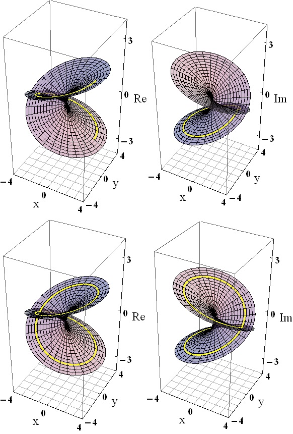

Using the technique in Section 1, we integrate the differential equation $\frac{dw}{dt}$ using the code

mysol=NSolve[theAzimuthalEq/.z->Exp[It],w[0]=w0,w,{t,0,2n PI}]

and obtain a numerical solution to the $2$-cycle branch of the square root in terms of the variable $t$ along the path $z=e^{it}$. So that we have: $$\bint w(t)dz=\bint w(t)\frac{dz}{dt}=\bint w(t) ie^{it}dt.$$ Or

myIntegral=NIntegrate[w[t] i Exp[it],{t,0,4 PI}].

And we of course obtain 0 since $2v^2$ is an entire function.

Figure 3: Mapping of complex plane under $z\to v^2$

We wish now to consider a slightly more complicated function where we can explicitly make the substitution $z=v^n$: $$w(z)=\displaystyle a+\frac{b}{z^{1/4}}+\frac{c}{z}+d z^{1/4}$$. so that we obtain $$\displaystyle w(v)=a+\frac{b}{v}+\frac{c}{v^4}+dv$$ and although $w(v)$ is already in it's power expansion, we wish to treat it as if we do not know this. That is, we wish to determine the power expansion of $w(v)$ using Laurent's Theorem: $$ \begin{align} w(v)&=\sum_{n=0}^{\infty} a_n v^n+\sum_{n=1}^{\infty}\frac{b_n}{v^n} \\ a_n &=\frac{1}{2\pi i}\oint \frac{w(v)}{v^{n+1}} \\ b_n &= \frac{1}{2\pi i}\oint w(v) v^{n-1} \end{align} $$ But we know Laurent's Theorem in $v$ will give us $w(v)$ and since $z=v^4$, we obtain the "fractional power series" in $z$ which is $w(z)$. And it turn out that any algebraic function can be written as a fractional power series. This is given by Newton-Puiseux's Theorem. In the case above, we were able to explicitly substitute $z=v^n$ to obtain a function in $v$. However, in most cases, we will not have an explicit expression for $w(z)$. For example, consider again the function reviewed in Section 1: $$ f(z,w)=a_1+a_2 w^2+(a_3+b_3z) w^4+(a_4+b_4 z) w^6+(a_5+b_5 z) w^8+a_6 z w^{10}+a_7 z w^{12}=0. $$ where we determined $w(z)$ ramified into three $4$-cycle branches. How do we determine the fractional power series for these branches? We have two methods. The most common method is the method of Newton Polygons which we will cover in another section. But in this section, we wish to show how Laurent's Theorem can be used to numerically compute the fractional power series for these branches. This exercise with give us a novel and unique insight into the branching geometry of these functions and help us better understand how to work with them. That is we wish to show given an $n$-cycle branch of an algebraic function $w(z)$, $$ \begin{equation} w_n(z)= \sum_{k=0}^{\infty} a_k (z^{1/n})^k+\sum_{k=1}^{\infty} \frac{b_k}{\left(z^{1/n}\right)^k} \\ a_k=\frac{1}{2n\pi i} \bint \frac{w_n(z)}{\left(z^{1/n}\right)^{k+n}} dz\\ b_k=\frac{1}{2n\pi i} \bint w_n(z)\left(z^{1/n}\right)^{k-n} dz \end{equation} $$ and recall these are branch integrals in which the integration path completely traverses the branch surfaces in an analytically continuous route. So that the first question becomes "how do we effect these integrations?" Well, we already know how to compute $w(z)$ along a branch contour from Section 1: we use the azimuthal and radial equations. So that we can do the same for the $n$-root branch. That is, we likewise compute azimuthal and radial equations for the quantity $u(t)=\left(z^{1/n}\right)^k$ and then integrate the above expressions through these results. We therefore integrate the following equations:

w[t]/.mynumer=NDSolve$\big[$w'[t]$\displaystyle \frac{dw}{dt}$,w[0]=$w_0$,{t,0,tend}$\big]$

u[t]/.mydenom=NDSolve$\big[$u'[t]==$\displaystyle\frac{1}{n \left(u^{1/n}\right)^{n-1}} \frac{dz}{dt}$,u[0]=$u_0$,w,{t,0,tend}$\big]$

However, we are confronted with deciding what initial conditions to use. In this example we have two $4$-cycle branches and therefore, for $z_0$ there are sixteen possible initial conditions: for each sheet on $w(t)$, we have four initial conditions to choose from on $u(t)$. It turns out with regards to computing the power expansions, it does not matter which one we choose from: we still obtain, in the case of $4$-cycle branches, four versions of the same power expansion $\displaystyle\sum_{n=-\infty}^{\infty} a_n \left(z^{1/4}\right)^n$ and we wish now to tabulate the first four terms of four of these expansions to experimentally confirm this and then attempt to explain algebraically why this is so.

From Section 1, we determined that the point $(1/2-1/2i,2.0043-0.2869i)$ was on the red branch of the function. We used that point as the initial condition for the azimuthal equation and integrated over the whole branch. We could then determine the remaining roots of $z_0=1/2-1/2i$ on this branch by simply finding $w(t_0+2k\pi i)$ from the solution of the azimuthal equation. However, these numerical results might be slightly off due to numerical errors. A better approach is to then compare these 4 values computed by numerical integration over the branch to roots calculated directly by NSolve which is much more accurate, and then use those roots as the initial starting points on the branch. We then compute the four roots to $\sqrt[4]{1/2-1/2i}$ and use those values for the starting points for that branch. We then tabulate four versios of the integrals $a_k$ and $b_k$ in equation (4) above according to which roots we used as the initial values for the integration and formed the resulting power series. The following Mathematica code does this (note the scroll bar):

Mathematica code

a = (2/3)*Exp[2*Pi*(I/3)];
theFunction = (Conjugate[a]*(a^2 - w^2))^4 - z*w^4*(a*(1 - Conjugate[a]^2*w^2))^4
myroots = w /. NSolve[theFunction == 0 /. z -> 1/2 - (1/2)*I, w];
xcod[t_] := (1/Sqrt[2])*Cos[t];
xdcod[t_] = D[xcod[t], t];
ycod[t_] := (1/Sqrt[2])*Sin[t];
ydcod[t_] = D[ycod[t], t];
tstart = -Pi/4;
tend = 31*(Pi/4);
rootnum = 1;
theorder = 4;
rnum = 1/Sqrt[2];
selectedroot = 1;
posbuffer = {};
wDeriv = Derivative[1][w][t] == ((-(D[theFunction, z]/D[theFunction, w]))*(xdcod[t] + I*ydcod[t]) /.
{w -> w[t], z -> xcod[t] + I*ycod[t]});
mysol = First[NDSolve[{wDeriv, w[tstart] == myroots[[selectedroot]]}, w, {t, tstart, tend}, MaxSteps -> 500000,
MaxStepSize -> 0.001]];
myw[t_] := Evaluate[w[t] /. mysol];
branchroots={myw[tstart],myw[tstart+2 PI],myw[tstart+4 PI],myw[tstart+6 PI]}; For[i2 = 1, i2 <= 4, i2++, theSelection = Select[myroots, Abs[#1 - branchroots[[i2]]] < 0.0001 & ];
If[Length[theSelection < 1], Print["error with roots"]; ]; pos = Position[myroots, First[theSelection]];
posbuffer = Append[posbuffer, pos]; ];
posbuffer = Flatten[posbuffer];
resultBuffer = {};
For[pbuf = 1, pbuf <= 4, pbuf++, mysol = First[NDSolve[{wDeriv, w[tstart] == myroots[[posbuffer[[pbuf]]]]}, w, {t, tstart, tend},
MaxSteps -> 500000, MaxStepSize -> 0.001]];
myw[t_] := Evaluate[w[t] /. mysol];
For[baseroot = 0, baseroot <= 3, baseroot++,
baseSol = NDSolve[{Derivative[1][f][t] == ((-rnum)*Sin[t] + I*rnum*Cos[t])/(theorder*f[t]^(theorder - 1)),
f[tstart] == Exp[(2*Pi*I*baseroot)/theorder]*(rnum*Exp[tstart*I])^(1/theorder)}, f, {t, tstart, tend}];
theBaseM[t_] := Evaluate[f[t] /. baseSol];
wOffset = 0; nmax = 5;
thealist1 = Table[n1 = NIntegrate[((xdcod[t] + I*ydcod[t])/theBaseM[t]^(j + theorder))*myw[wOffset + t], {t, tstart, tend},
MaxRecursion -> 20];
If[Length[n1] == 1, {j, First[N[(1/(2*theorder*Pi*I))*n1]]}, {j, N[(1/(2*theorder*Pi*I))*n1]}],
{j, -nmax, nmax}];
newlist = thealist1; tolerance = 10^(-6);
thevals = Select[newlist, Abs[#1[[2]]] > tolerance & ];
For[i = 1, i <= Length[thevals], i++,
If[Abs[Re[thevals[[i,2]]]] < tolerance || Abs[Im[thevals[[i,2]]]] < tolerance,
{If[Abs[Re[thevals[[i,2]]]] < tolerance, thevals[[i,2]] = I*Im[thevals[[i,2]]], thevals[[i,2]] =
Re[thevals[[i,2]]]]; }]; ];
truncatedSeries = Sum[thevals[[n,2]]*(z^(1/theorder))^thevals[[n,1]],
{n, 1, Length[thevals]}];
Print["Roots: ", {posbuffer[[pbuf]], baseroot}, " Series: ", truncatedSeries];
resultBuffer = Append[resultBuffer, {{posbuffer[[pbuf]], baseroot}, " Series: ", truncatedSeries}]; ]; ];
resultBuffer

Using the first branch sheet of the function and the four branch sheets of $\sqrt[4]{z}$, we obtain the first four terms of the following series where the expression (n,m) represents beginning the integration on the n'th sheet of the red branch and m'th sheet of $\sqrt[4]{z}$:

$$ \begin{equation} \begin{aligned} (1,0): & & \frac{-0.25i}{z^{1/4}}+(0.6949-0.4012i)z^{1/4}-(0.1868+0.1078i)z^{3/4}+0.1098 i z^{5/4}\\ (1,1): & & \frac{2.25}{z^{1/4}}-(0.4012+0.6936i)z^{1/4}+(0.1079-0.1868i)z^{3/4}+0.1098 z^{5/4} \\ (1,2): & & \frac{2.25i}{z^{1/4}}-(0.695-0.4012i)z^{1/4}+(0.1868+0.10788i)z^{3/4}-0.1098i z^{5/4} \\ (1,3): & & -\frac{2.25}{z^{1/4}}+(0.4012+0.6949i)z^{1/4}-(0.1078-0.1868i)z^{3/4}-0.1098 z^{5/4} \end{aligned} \end{equation} $$

And we need to study these four solutions carefully because they are four ways of representing the same $4$-cycle power series and any one can be used to generate the entire red branch described in Section 1 although more than four terms of the power series would probably be needed to generate an accurate plot of the function.

The first thing to note about the series is the $\displaystyle\frac{k}{z^{1/4}}$ term which means of course $\displaystyle \lim_{z\to 0} w(z)=\infty$ for this branch. This was mentioned in Section 1 where we truncated the graph of the function for a better looking plot. The function $w(z)$ will tend to infinity at the origin whenever $a_n(0)=0$ as is the case with this function. However the remaining branches do not tend to infinity and if we computed the series for the two remaining $4$-cycle branches, both would contain no negative powers of $z^{1/4}$.

The second feature of these series is that they are the same $4$-cycle series and we can interpret the series in two ways:

1. Using the principal branch of $z^{1/4}$: In this case we let $\quad z^{1/4}=r^{1/4}e^{it/4},\quad -\pi\le t\lt \pi$ so that if we choose one of the series above and let $\displaystyle s_1=\sum_{n=0}^{\infty}a_n \left(z^{1/4}\right)^n$ then $\displaystyle s_k=\sum_{n=0}^{\infty} a_n\left(e^{2k\pi i/4}\right)^n \left(z^{1/4}\right)^n,\quad k=1,2,3$ with $s_2, s_3,s_4$ the remaining series reported above. We would then need to generate four separate single-valued sheets of the branch. In this case, these sheets are easily plotted with the standard Plot3D function and then stitched together via the function Show[{p1,p2,p3,p4}].
2. Treating $z^{1/4}$ as a $4$-cycle branch: In this case, we could devise the azimuthal equation over $z^{1/4}$ to obtain its analytically continuous version and then substitute that function into a single series and generate the plot as described in Section 1.

Figure 4 gives some practical comparison between the plot generated by the azimuthal equations in Section 1 and a plot generated by ten terms of the power series in this section using the principle-valued method described above.

Figure 4: Comparison of azimuthal plot (red) and principle-valued plot (green)