Algebraic functions, iterated exponentials and polynomial systems: Section 11: Riemann Surfaces

$$ \newcommand{\bint}{\displaystyle{\int\hspace{-10.4pt}\Large\mathit{8}}} $$

Mapping a double cover of the complex plane to a torus

Note: A Mathematica notebook of this topic in the form of a slide-show was presented at the 2017 Wolfram Tech conference and is available for download. The slide show includes an animation of bending the double-cover into a torus. Please note the file is over 350Mb due to the large amount of graphics and will take a bit to load. Once loaded into Mathematica, again, the slide show will take about a minute to set up before being available to run. Attempting to run the show before this time will result in a "Mathematica not responding" message. Give it time and the message will go away. Link to slide show here: Mapping a double cover to a torus

In this section we describe how to map a double cover of the complex plane onto a genus 1 Riemann surface, a torus. We will use the following.

Figure 1

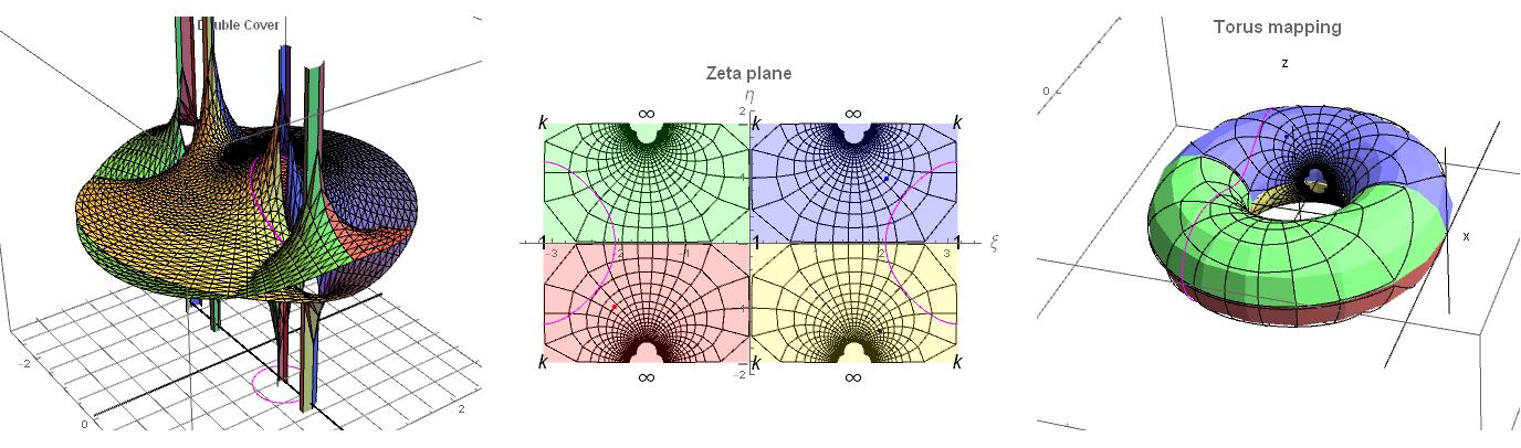
In the first plot at the left, we have a small section of the real part of the function $\displaystyle g(z)=\frac{A}{\sqrt{(1-z^2)(k^2-z^2)}}$ which is analytic and double-valued for all values of $z$ except at the branch points. We will use the first plot as the icon of the double cover as we map two copies of the complex plane to the torus and remember $g(z)$ is actually made up of a real and imaginary part extending in all directions over the complex plane out to infinity. Next, we use a set of Schwarz-Christoffel transformations to map the covers to the rectangular region in the $\zeta$ plane shown in the center plot which we call the $\zeta$-cover. We then continuously contort the $\zeta$-cover into the torus show in the third plot. The covers are color-coded for each half-plane. For example, the blue surface of $g(z)$ in the first plot is mapped to the blue rectangle in the $\zeta$-cover, and then this rectangle is mapped to the blue quarter-section of the torus in the third plot.

Mapping of the double cover to the $\zeta$-plane is done with the Schwarz-Christoffel transformation and it is this transformation we need to study next.

Schwarz-Christoffel Transformation

Suppose that P is a polygon with vertices $w_1,\cdots,w_k$ in the anticlockwise direction,with corresponding right turns of angles $\theta_1\pi,\cdots,\theta_k \pi$ respectively, where $−1 < \theta_1, \cdots, \theta_k< 1$. Then there exists a function of the form $$ \zeta(z)=A \int_0^z (w-x_1)^{\theta_1}\cdots (w-x_k)^{\theta_k} dw+B $$ where $A,B\in \mathbb{C}$ that maps the upper half plane H one-to-one and conformally onto the interior of P,with $\zeta(x_1) = w_1, \cdots, \zeta(x_k) = w_k$.

And in our particular application, we wish to map the upper half plane to the rectangle

Figure 2

with $$p=\int_0^{\pi} \frac{1}{2+\cos(t)}dt. $$

And starting at the point $-\pi/2+ip$ and going counter-clockwise we make left turns of $\pi/2$, we then have $\theta_i=-\pi/2$ and we can choose $x_1=1, x_2=-1, x_3=k, x_4=-k$ with $k$ real and $|k|>1$. We then have $$ \zeta(z)=A\int_0^z \frac{1}{\sqrt{(1-w^2)(k^2-w^2)}}dw+B. $$

The constant B is a translation so for now, we set it to zero and then later move the polygon as needed by adjusting B. Our objective now is to find constants A and k, such that f(z) maps the upper half-plane to the rectangle described above. These can be determined by considering the four simultaneous integral equations: $$\begin{align} A\int_0^{-k} \frac{dt}{\sqrt{(1-t^2)(k^2-t^2)}}&=-\pi/2+ip \\ A\int_0^{-1} \frac{dt}{\sqrt{(1-t^2)(k^2-t^2)}}&=-\pi/2\\ A\int_0^{1} \frac{dt}{\sqrt{(1-t^2)(k^2-t^2)}}&=\pi/2 \\ A\int_0^{k} \frac{dt}{\sqrt{(1-t^2)(k^2-t^2)}}&=\pi/2+ip \end{align} $$

Looking at (3) we have immediately, $$\begin{equation} \displaystyle A=\frac{\pi}{2 \int_0^1 \frac{dt}{\sqrt{(1-t^2)(k^2-t^2)}}}. \end{equation} $$ And if we subtract (3) from (4) we obtain $\displaystyle A\int_1^{k} \frac{dt}{\sqrt{(1-t^2)(k^2-t^2)}}=ip$. Using this expression and (3) we can write: $$ \frac{1}{p}\int_1^k \frac{dt}{\sqrt{(t^2-1)(k^2-t^2)}}=\frac{2}{\pi} \int_0^1 \frac{dt}{\sqrt{(1-t^2)(k^2-t^2)}} $$ and numerically solve for $k$ and then using (5), solve for A. Keep in mind the integrals are improper (and convergent) and we need to integrate over an analytically-continuous path between the singular points. Usually, this is over the principal branch.

The following Mathematica code computes these values:
```
rhoMax = NIntegrate[1/(2 + Cos[a]), {a, 0, \[Pi]}];
myf1[a_?NumericQ] := 
 NIntegrate[1/rhoMax 1/Sqrt[(t^2 - 1) (a^2 - t^2)], {t, 1, a}]
myf2[a_?NumericQ] := 
 NIntegrate[2/\[Pi] 1/Sqrt[(1 - t^2) (a^2 - t^2)], {t, 0, 1}]

thek = a /. FindRoot[myf1[a] - myf2[a] == 0, {a, 2}]
bigA = 1/myf2[thek]
```
From which we find $A\approx 1.53126$ and $k\approx 1.6984$

Integrating over a half-plane

Although Mathematica has built-in functions to compute a Schwarz-Christoffef integral in terms of EllipticF, we obtain a more complete understanding of integrating over multi-valued functions if we design our own algorithm to compute this integral. We already have the technique to do so from earlier sections of this site: we form the associated differential equation, solve it via NDSolve, then integrate the solution over the desired path. And having the ability to plot the solution path over the real or imaginary surface of a cover, gives us an intuitive confidence that we are integrating over the correct surface of this multivalued function. Readers are encouraged to review the section on plotting algebraic functions for a review of this method.

The following Mathematica code computes the value of the integral for z=1+i over the blue upper half-plane:

(* express function in it's algebraic form *)
theA = 1.5312624348967;
theK = 1.6983963730242;
theFunction = theA^2 - (1 - z^2) (theK^2 - z^2) w^2;

(* integrate to 1+1 i over the blue covering (the principal-valued \
root *)
thez[t_] := t + t I;
tend = 1;
(* the choice of \[Sqrt](k^2) will determine which cover to integrate \
over *)
theroots = w /. NSolve[theFunction == 0 /. z -> thez[0]];
wstart = theroots[[2]];
wDeriv = w'[
    t] == ((-(D[theFunction, z]/D[theFunction, w]) (D[thez[t], 
         t])) /. {w -> w[t], z -> thez[t]});
myazsol = First[NDSolve[{wDeriv, w[0] == wstart}, w, {t, 0, tend}]];
myCentralTrace[t_] = Evaluate[Flatten[w[t] /. myazsol]];
blueTrace = 
 ParametricPlot3D[{Re[z], Im[z], Re[myCentralTrace[t]]} /. 
   z -> t + t I, {t, 0, 1}, PlotStyle -> Red]

(* now integrate the solution over the path of integration *)
n1 = NIntegrate[myCentralTrace[t] D[thez[t], t], {t, 0, tend}]
zetaBluePoint = 
  Graphics[{Blue, PointSize[0.015], Point[{Re[n1], Im[n1]}]}];
zetaBluePointTranslated = 
  Graphics[{Blue, PointSize[0.015], 
    Point[{Re[n1 + \[Pi]/2], Im[n1]}]}];
(* as a check of the computations, compare the results to EllipticF *)


ellipticValue = N[theA/theK EllipticF[ArcSin[thez[tend]], 1/theK^2]];
Print["Value by integration: ", n1];
myk = NIntegrate[1/(2 + Cos[t]), {t, 0, \[Pi]}]
Print["EllipticF value:      ", ellipticValue];

We obtain $\zeta_b(1+i)=0.492972 + 0.970237i$

Plotting the integration results to the $\zeta$-plane

We can then integrate over a grid of points for each half-plane cover, that is, over the red, blue, green and yellow covers. And then map the values of $\zeta(z)=\xi+\eta i$ in the $\zeta$-plane with one addition: we need to translate the values by $\pm \pi/2$. This is illustrated in the next plot where we have also plotted the mapping of the ramified contour around the singular point z=1 and also the mappings for z=1+i over the red and blue sheets as the red and blue points in their corresponding red and blue sections of the plot. The red and blue points illustrate an important point of this mapping: for each value of z in the z-plane, there are two distinct points in the $\zeta$-plane. This is the beginning of resolving a double-valued function into a single valued function of the points in the $\zeta$-plane and then of the points $p$, over the torus.

Figure 3
Bending the $\zeta$-cover into a torus

We now wish to map the $\zeta$-cover into a torus. If we are given the equations of the torus in the xyz-plane by $$ \begin{align*} x(\alpha,\phi)=[R+\rho \cos(\alpha)]\cos(\phi) \\ y(\alpha,\phi)=[R+\rho \cos(\alpha)]\sin(\phi) \\ z(\alpha,\phi)=\rho \sin(\alpha) \end{align*} $$ where R is the radius of the torus from its center to the center of the tube and $\rho$ is the radius of the tube, then the mapping from $\xi$ and $\eta$ in the $\zeta$ plane to $\alpha$ and $\phi$ is given by $$ \begin{align*} \xi &= \phi \\ \eta &= \int_ 0^{\alpha}\frac {\rho} {R + \rho \cos(t)}dt \end{align*} $$ so that as $\alpha$ and $\phi$ both vary from $-\pi$ to $\pi$, $\xi$ varies from $-\pi$ to $\pi$ and $\eta$ varies from $0$ to $p$ where $$ p=\int_ 0^{\pi}\frac {\rho} {R + \rho \cos(t)}dt $$

A plot of this mapping onto the torus can be viewed with AFRender. Choose 'Torus' and then drop down the ring table and check the contour box to illustrate the contours over the torus.
Characterizing contours over the torus

Now that we can map the double cover onto the torus, we wish to study how various contours in the $z$-plane are mapped and to attempt to identify equivalent contours, that is contours homomorphic to one another. However, before we begin traversing through the function branch sheets, we should determine the monodromies or branch cycles around each singular point. This is relatively easily accomplished by forming the azmithual equation (see earlier sections) and following a circular path around a singular point. We then check the winding numbers for paths to return to their starting points within numerical accuracy. This is of course not a rigorous determination of monodromy and can lead to errors, but for relatively well-behaved functions even of high degree, the method has proven to be very successful by comparing the subsequent numerical results to expected results such as with the Residue Theorem. The result of this analysis leads to a monodromy or branch table which gives a list of the singular points followed by the branch cycles. For a single-cycle we have the notation of $\{k\}$ which is a root number associated with the cycle. For a $2$-cycle, we would obtain $\{k,j\}$ and so forth for the remaining cycles. When we do this, we obtain the following: $$ \left( \begin{array}{cccc} 1 & -1.0000000 & \begin{array}{cc} \{1,2\} \\ \end{array} & \\ 2 & 1.0000000 & \begin{array}{cc} \{1,2\} \\ \end{array} & \\ 3 & -1.6983964 & \begin{array}{cc} \{1,2\} \\ \end{array} & \\ 4 & 1.6983964 & \begin{array}{cc} \{1,2\} \\ \end{array} & \\ 5 & \infty & \begin{array}{c} \{\{1\},\{2\}\} \\ \end{array} & \\ \end{array} \right) $$ From the table, we see the function fully-ramifies into $2$-cycle branches at the four finite singular points. This means of course that a closed analytically-continuous path over the double cover, $g(z)$ around each of these points will have a winding number of $2$.

Now consider the contours in Figure 4.
Figure 4
1. First Contour (shown as the pink contours in Figure 5 below)